Solve Equations numerically with Newton’s Method

Trust me I’m an engineer

There will be a time when we want to solve equation as part of our program and algebra simply just fails (Or we failed algebra — more likely).

Newton’s Method

Those times are ideal to whip out good old Newton’s Method to provide a good enough answer. It is based on deceptively simple but enormously useful observation that we can get a better answer (X(n+1)) from a previous answer (Xn).

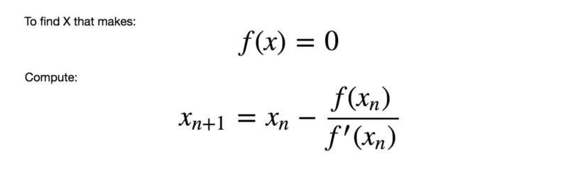
As we progress, next value of X will be closer to the answer and we can stop computing when current X produced f(x) that is closed enough to 0.

Step 1: Confirms the Variable

The problem we are going to solve is to find Internal Rate of Return with Annuity. Which bears this equation

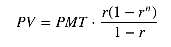
Biggest plot twist here is that we want to solve for (r) rather than (PV), so this is not simply “plugging value and it works” business.

It is quite easy to loose track of what is the variable to solve for. Let’s confirm that there is only a single value to find while others are just given parameters.

Given the equation above. We want to solve for (r), given all the other values of (PV,PMT,n).

Step 2 : Rearrange Equation

Newton’s Method is specialized to find X that makes f(x) = 0. This is not quite how the equation is right now. Let’s move things around.

A Python code for f(r) would be this def. It generates a function that accepts (r) as variable, given (n,PV,PMT) as a fixed parameter.

def f(n,PV,PMT):
    return lambda r:r * (1 - r**n) / (1 - r) - PV/PMT

Step 2: Find Derivative of f(x)

The f’(x) part in Newton’s Method equation is a derivative of f(x). While not particularly hard to work out by hand, it is much simpler and fun to paste whole equation into Wolfram Alpha

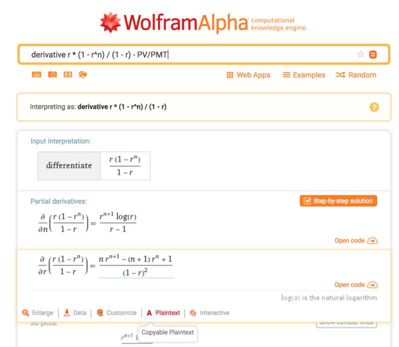
Again, try not to confuse which one is the variable. In this case we need (d/dr).

A Python code for f_prime(r) would be this def. It generates a function that accepts (r) as variable, given (n) as a fixed parameter. PV and PMT are not necessary as it is eliminated by derivative. They are left here just for consistency with f(r).

def f_prime(n,PV,PMT): 
    return lambda r: (n*r**(n + 1) - (n + 1)*r**n + 1)/(1 - r)**2

Step 3: Graph Equation and Slope

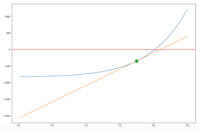
To provide better context and sanity check that both equations are correct. This is also helpful in visualizing a good initial estimate.

Pick a parameter of (n,PV,PMT), graph 2 things

1. A graph of f(r)
2. A graph of tangent line at a given (x_test). In this case (x_test) = 1.7

Step 4: Compute

Everything’s set. So let’s code up Newton’s Method itself.

def solve(f,f_prime,x0,tolerance=1e-4,maxiter=200):
    xn = x0
    for i in range(maxiter):
        #Very close to 0 now
        if abs(f(xn)) < tolerance:
            return xn
        
        xn = xn - f(xn) / f_prime(xn)
        
    raise Exception("Does not converge")

Now plug in all the hard work to find that precious (r)

n, PV, PMT = 10,10000,12
x_start = 1.01

solved_r = solve(f(n, PV, PMT), f_prime(n, PV, PMT), x_start)

And the value of (r) in this case is

solved_r = 1.8081007002833853

For those who’s interested in using a standard package can use SciPy (scipy.optimize.newton). Note that it will help only with this step. Finding f(r) and f_prime(r) is still a required manual work.

Step 5: Check Your Work

Good Engineers check their work. That’s also what we are going to do here.

Here is the PV equation that we started with coded in Python

def PV(n,r,PMT):
    return PMT * r * (1 - r**n) / (1 - r)

Plugged in the (solved_r) computed above to get the result that we expected (10,000).

PV(10, solved_r, 12) # Yields 10000.000000180908

Reference

For those who are curious to see the notebook that generates all the equations and graphs, please see link below.

Microsoft Azure Notebooks - Online Jupyter Notebooks
Provides free online access to Jupyter notebooks running in the cloud on Microsoft Azure.notebooks.azure.com